From Learning and Evolution to Data Science2019-11-16T00:56:50.778Zhttps://dracodoc.github.io/dracodocHexoReactive in Shinyhttps://dracodoc.github.io/2019/11/15/shiny-reactive/2019-11-16T00:42:58.000Z2019-11-16T00:56:50.778ZIntro
In preparing an invited talk on Shiny, I organized my experience and notes on reactive programming, and found the storyline I developed may actually be a good alternative compare to the usual tutorials on this topic. Thus I’m expanding the talk slides into a blog post and sharing it here.
Programming for User Interface: Event Driving programming
Programming user interface is different from some other domains, because user interface need to respond to user input and you don’t know when that will happen. Usually this means you write some logic for some possible situations, and there will be a maintained loop watching for user input, and trigger the appropriate logic when the input happens.
In desktop application development, the common pattern is Event Driven programming. User input will generate some event, and the event object have information about the input. You can write code for specific event and conditions, “register” the event to the system (the programming framework), and the system will trigger the code. Here the framework handle the details about event, registering, triggering, and developer only need to write code for event handling.
This pattern is straightforward and not hard to understand. Shiny support this pattern too (observeEvent, note sometimes you may see code examples using observe, which is a low level API and I believe usually there is no real reason for you to use observe instead of more friendly observeEvent.) since it’s a good approach for certain use cases.
There is a slight difference in Shiny observeEvent though. You can think it is observing data changes in the target, not really some event object (it’s possible in the underlying level implementation of Shiny framework something can be called as event object, but I think this way of understanding will help to recognize the difference and connection to the reactive programming topic later). For example, an actionButton click actually just increase its return value by 1, and that value change can trigger some observeEvent code. You can even write something like observeEvent(1, {...}), just the code will only execute once and not again.
If we think observeEvent observe data changes, it can be triggered by any kind of change, including user input (which will change the value input$widget_id), reactive expressions(we will discuss it next).
Summary: observeEvent observe data changes in target expression, run the code once anything changed (there are more options control the fine details, like whether to run in initialization, if to ignore NULL etc, see help page of observeEvent).
observeEvent: data changes ---trigger---> event handling code
Note the official tutorials differentiate event observer and reactive expressions mainly by side effect/calculated values. In my experience this difference is less useful than the difference of source/target of changes, the latter often determined which one you need to use, and you can have side effect in reactive expression in some valid user cases. After all, anything interacting with outside world is side effect, and we need to interact with outside world a lot in user interface programming.
If your reactive expression only returned some changed values and that didn’t reflect to GUI, why were the changes needed? if it did reflect to GUI, that’s still side effect, just shiny framework did the plumbing work and made the changes so the reactive expression didn’t look like did anything imperative.
More relevantly, should use the design principle of cohererant and loose coupling. let related event update together. if you have multiple control for one final value, better use a reactive expression instead of multiple observer.
In this post my perspective is to introduce reactive pattern by comparing with event driving programming.
A reactive expression/value will automatically update itself triggered by data changes in source of changes. This automatical update is handled by Shiny framework, thus require less manual work and appears to be more magical to developers.
Reactive Expression: all reactive values inside become source of changes
observeEvent is triggered by data changes in the target expression, while a reactive expression update is triggered by all data changes in all reactive values inside the expression, and you don’t need to register them explicitly.
reactive({
    ...
    Shiny UI reactive values like input$checkbox
    reactive values defined by reactiveValue()
    other reactive expression()
})
dynamic data 1
dynamic data 2  ==> expression reevaluate
dynamic data 3
Note:
Reactive expression look like a function, use like a function. Thus you reference it with () for the updated value, transfer it without () in some other scenarios (like Shiny module) when you are using the expression itself but not going to use the updating value immediately.
Reactive Expression Vs observeEvent
Compare to observeEvent, you can establish multiple -> one data update relationship in reactive expression without explicit registering, thus this is a prefered way if it met all your needs.
In observe) help page, there are some official comparison for these two, mainly focused on:
it doesn’t yield a result and can’t be used as an input to other reactive expressions. Thus, observers are only useful for their side effects (for example, performing I/O). Another contrast between reactive expressions and observers is their execution strategy. Reactive expressions use lazy evaluation; that is, when their dependencies change, they don’t re-execute right away but rather wait until they are called by someone else. Indeed, if they are not called then they will never re-execute. In contrast, observers use eager evaluation; as soon as their dependencies change, they schedule themselves to re-execute.
All these are definitely valid points, but I think the deciding factor for choosing one of them should be just how you want to arrange the source of changes and eager vs lazy evaluation. With observeEvent you need to be more explicit and have more control, with reactive expression you “let it go” and everything will work smoothly if it fit the pattern.
Reactive Values
One real limit with reactive expression is that you cannot modify its value arbitrarily. It can update when source of changes changed, but always change with same expression. When you need to modify the dynamic data from another source/place/time, you need reactive values.
Thus you have more control and more responsibilities with reactive values
- read reactive value inside reactive expression
  - value change ==> expression reevaluate
- write reactive value inside reactive expression
  - expression reevaluate ==> value updated
- read/write same reactive value inside reactive expression?
  - that will cause an infinite loop
Shiny input/output as reactive special cases
input value (input$slider_value) are reactive values driven by user input
output code (renderPlot) create reactive scopes like reactive expression
return value used immediately
if you need to reuse the value, just create a reactive expression and reference it
Error: Operation not allowed without an active reactive context
Every reactive value inside a reactive domain (like inside a reactive expression, output code which is reactive domain implicitly) get registered by Shiny framework behind the scene so their changes can be monitored. Thus using a reactive value outside of reactive domain will raise this error.
If you do need to inspect the value in debugging, or you want to read the value but don’t want the value update trigger reactive expression reevaluation, you can use isolate.
When more controls are needed
The components above can be used to create sophisticated dynamic systems. However sometimes the order of changes may not be ideal with these rules.
One simple case is that your downstream reactive expression/value may not have valid upstream value yet when the app UI is initialized. You can use req to hold off the related UI widget rendering before the upstream value is ready.
Sometimes you have multiple widgets updating at the same time driven by some changes, and some widget always update slower, this may cause problems.
For example, DT is one of my favorite package and I used it extensively in my app, often using the table selection to control other parts of app. When a DT table was updated, the row information will update after the whole table render finish, which is often the slowest one if other widgets are updating at the same time. I may have a plot is depending on some row selection value, so there will be a short time period when the row selection value are not valid and plot will render with the invalid value. Once the table finished update it will be corrected.
In the beginning I tried to use priority levels to adjust the order, but that seemed never work.
Instead you can use freezeReactiveValue, which will hold off downstream changes until the last second, so the plot will not render with the invalid value.
]]>
<h2 id="Intro"><a href="#Intro" class="headerlink" title="Intro"></a>Intro</h2><p> In preparing an invited talk on Shiny, I organized my experience and notes on reactive programming, and found the storyline I developed may actually be a good alternative compare to the usual tutorials on this topic. Thus I’m expanding the talk slides into a blog post and sharing it here.</p>
Make link button with Shiny functionshttps://dracodoc.github.io/2017/06/03/shiny-link-button/2017-06-04T02:25:27.000Z2017-06-04T02:33:09.772ZYou can customize Shiny to a much greater extent if you knew Shiny UI functions just generate html codes. You can make a link button with creative use of Shiny functions.
]]>
<p>You can customize Shiny to a much greater extent if you knew Shiny UI functions just generate html codes. You can make a link button with creative use of Shiny functions.<br>
Color Sync in multiple ggplotshttps://dracodoc.github.io/2017/04/08/color-sync-gg/2017-04-08T12:30:34.000Z2017-06-04T01:44:31.369ZThis is a summary about my experience on synchronize colors in multiple ggplots of same dataset.
]]>
<p>This is a summary about my experience on synchronize colors in multiple ggplots of same dataset. </p>
rCartoAPI - call Carto.com API with Rhttps://dracodoc.github.io/2017/01/21/rCarto/2017-01-21T22:04:26.000Z2017-01-22T01:47:44.335ZSummary
My experience with Carto.com in creating web map for data analysis
I wrote a R package to wrap Carto.com API calls
Some notes on my experience of managing Gigabyte size data for mapping
Introduction
Carto.com is a web map provider. I used Carto in my project because:
With PostgreSQL, PostGIS as backend, you have all the power of SQL and PostGIS functions. With Mapbox you will need to do everything in JavaScript. Because you can run SQL inside the Carto website UI, it’s much easier to experiment and update.
The new Builder let user to create widgets for map, which let map viewers select range in date or histgram, value in categorical variable, and the map will update dynamically.
Carto provide several types of API for different tasks. It’s simple to construct an API call with curl but also very cumbersome. You also often need to use some parts of the request response, which means a lot of copy/paste. I try to replace all repetitive manual labor with programs as much as possible, so it’s only natural to do this with R.
There are some R package or function available for Carto API but they are either too old and broken or too limited for my usage. I developed my own R functions for every API call I used gradually, then I made it into a R package - RCartoAPI.
upload local file to Carto
let Carto import a remote file by url
let Carto sync with a remote file
check sync status
force sync
remove sync connection
list all sync tables
run SQL inquiry
run time consuming SQL inquiry in Batch mode, check status later
So it’s more focused on data import/sync and time consuming SQL inquiries. I have found it saved me a lot of time.
Carto user name and API key
All the functions in the package currently require an API key from Carto. Without API key you can only do some read only operations with public data. If there is more demand I can add the keyless versions, though I think it will be even better for Carto to just provide API key in free plan.
It’s not easy to save sensitive information securely and conveniently at the same time. After checking this summary and the best practices vignette from httr, I chose to save them in system environment and minimize the exposure of user name and API key. After reading from system environment, the user name and API key only exist inside the package functions, which are further wrapped in package environment, not visible from global environment.
Most references I found in this usage used .Rprofile, while I think .Renviron is more suitable for this need. If you want to update variables and reload them, you don’t need to touch the other part in .Rprofile.
When package is loaded it will check system environment for the user name and API key and report status. If you modified the user name and API key in .Renviron, just run update_env().
Some tips from my experience
csv column type guessing
Carto by default will set csv column type according to column content. However sometimes column with numbers are actually categorical, and often there are leading 0s need to be kept. If Carto import these columns as number, the leading 0 information is lost and you cannot recover it by changing column type later in Carto.
Thus I will add quote for the columns that I want to keep them as characters, and use parameter quoted_fields_guessing as FALSE by default. Then Carto will not guessing type for these columns. We still want the field guessing on for other columns, especially it’s easier that Carto recognize lon/lat pair and build the geom automatically. write.csv will write non-numeric columns with quote by default, which is what we want. If you are using fwrite in data.table, you need to set quote = TRUE manually.
update data after a map is created
Sometimes I may want to update the data used in a map after the map has been created, for example there are more data cleaning needed. I didn’t find a straightforward way to do this in Carto.
One way is to upload the new data file with new name, then duplicate the map, change the SQL call for the data set to load the new data table. There are multiple manual steps involved, and there will be duplicated maps and data sets.
Another way is to set map using a sync table to a remote url, for example dropbox shared file. Then you can update the file in dropbox, let Carto to update the data. If the default sync interval is too long, there is force_sync function in package to force immediate sync. Note there is a 15 mins wait from last sync before force sync can work.
It also worth note that by copying new version of data file into the local dropbox folder to override the old version will update the file and keep the sharing link same.
upload large file to Carto
There is a limit of 1 million rows for single file upload to Carto. I have a data file with 4 million rows, so I have to split it into smaller chunks, upload each file, then combine them with SQL inquries. With the help of rdrop2 package and my own package, I can do all of these automatically, which make it much easier to update the data and run the process again.
Compare to upload huge local file directly to Carto, I think upload to cloud probably is more reliable. I chose dropbox because the direct file link can be inferred from the share link, while I didn’t find a working method to get direct link of google drive file.
To run the code below you need to provide a data set. Then the verification part may need some column adjustment to pass.
library(data.table)
# setup rdrop2
devtools::install_github('karthik/rdrop2')
library(rdrop2)
drop_auth()
# provide your data set here
target <- data.table(dataset)
# use small size to test workflow first, change to full scale later
chunk_size <- 200
name_prefix <- "bfa_sample"
file_count <- ceiling(target[, .N] / chunk_size)
# generate this to be used later. note no ".csv" part here
res <- drop_share(drop_search(file_name_list[i])$path, short_url = FALSE)
file_urls[i] <- res$url
}
# setup dropbox sync, wait complete, get table id
for (i in seq_along(file_urls)) {
res <- url_sync(convert_dropbox_link(file_urls[i]))
}
# check result
tables_df <- list_sync_tables_df()
My case need to upload 4 200M files. Any error in the network or Carto server may prevent it finish perfectly. Upon checking the sync table I found the last file sync is not successful. I tried force sync it but failed, so I just use this code to upload and sync that file again.
# need both file_path and file_name
file_path <- "your file path"
file_name <- "your file name"
drop_upload(file_path)
res <- drop_share(drop_search(file_name)$path, short_url = FALSE)
file_url <- res$url
# setup dropbox sync, wait complete, get table id
res <- url_sync(convert_dropbox_link(file_url))
dt <- list_sync_tables_dt()
merge uploaded chunks with Batch sql
With all data files uploaded to Carto, now we need to merge them. Because I tested with small size sample first, I can test my sql inquiry in the web page directly (click a data set to open the data view, switch to sql view to run sql inquiry). After that I run the sql inquiry with my R package. With everything works I change the data set to the full scale data and run the whole process again.
I used a template for sql inquiries because I need to apply them for small sample file first, then larger full scale file later. With a template I can change the table name easily.
Carto expect a table matching some special schema to work, including a cartodb_id column. When you upload a file into Carto, Carto will convert the data automatically in the importing process. Since we are creating a new table by sql API directly, this new table didn’t go through that process and is not ready for Carto mapping yet. We need to drop the cartodb_id column, run cdb_cartodbfytable function to make the table ready. Only after this finished you can see the result table in the data set page of Carto.
The sql inquiries we used here need some time to finish. With rCartoAPI you can run the inquiries and check the job status easily.
# pattern of uploaded file name
file_name_pattern <- "data_set"
tables_dt <- list_sync_tables_dt()
# get the full table name for uploaded files in Carto
sql_inquiry_dt("select * from data_set_all limit 2")
sql_inquiry_dt("select count(*) from data_set_all")
# run batch job 2, cartodbfy
job_2 <- sql_batch_inquiry_id(inq[[2]])
sql_batch_check(job_2)
# check result
sql_inquiry_dt("select * from data_set_all limit 2")
After this I can create map with the merged data set. However the map performance is not ideal. I learned that you can create overviews to improve performance in this case.
So I can drop the overviews for the uploaded chunks, which were created automatically in importing process but we don’t need it. Then create overview for the merged table.
Later I found I want to add a year column that work as categorical instead of numerical. Even this simple process is very slow for table this large. I have to use Batch sql inquiry for this. I also need to update the overview for the table after this change to data.
]]>
<h2 id="Summary"><a href="#Summary" class="headerlink" title="Summary"></a>Summary</h2><ul>
<li>My experience with Carto.com in creating web map for data analysis</li>
<li>I wrote a R package to wrap Carto.com API calls</li>
<li>Some notes on my experience of managing Gigabyte size data for mapping</li>
</ul>
RStudio addin - extend RStudio in your wayhttps://dracodoc.github.io/2016/08/10/rstudio-addin/2016-08-10T17:57:23.000Z2016-08-30T17:55:16.329ZRStudio addins - first attempt
Recently I found RStudio began to provide addin mechanism. The examples looked simple, and the addin API easy to use. I immediately started to try writing one by myself. It will be a good practice project for writing R package, and I can implement some features I wanted but not in RStudio’s high priority list.
My first idea came from a long time frustration of using Ctrl+Enter to run current statement in console. With ggplot code like this, Ctrl+Enter only send one line with your cursor.
I submitted a feature request for this to RStudio support, though I didn’t expect it to be implemented soon since they must have lots of stuff in list.
After a little bit research on how R can recognize multiple line statement to be single statement, I felt the problem was not easy but doable.
R know a statement is not finished yet even with newline if it found
a string started with quotation mark
an operator like +, /, <- in the end of line
a function call started with (
I started to write regular expressions and work on the addin mechanism. After some time I began to test on sample code, then I found RStudio can send multiple line statement with Ctrl+Enter correctly!
Turned out I just upgraded RStudio to the latest preview beta version because of requirement of addin development, and the latest preview version implemented my feature suggestion already. I knew it could be easy from RStudio angle because RStudio has analyzed every line of code, and should have many information readily available.
mischelper
With my initial target crossed off, I tried to find some other usages that could use an addin.
First candidate came from my experience of copying some text from PDF as notes: I’d like to remove the hard line breaks from PDF. To do this I need to separate the hard word wrap from the normal paragraphs. With some experimentations on regular expressions this was done in a short time. I also added option to insert empty line between paragraphs.
I felt the remove hard line break feature is too trivial to be an independent addin, so I added yet another trivial feature: flip the windows path separator \ into /. Thus I can copy a file or folder full path in Total Commander, paste it into R script with one click.
Still not satisfied, I found a really useful function later: if you want to do a simple benchmark or measuring time spent on code, the primitive method is to use proc.time(). Or you could use the great microbenchmark package, which would run the code several times to get better statistics. To use microbenchmark, you need to wrap your code or function like this:
microbenchmark::microbenchmark({your code or function}, times = 100)
It’s not hard if you are just measuring a function, but I found I wanted to measure a code chunk instead of function in most times. Because it’s harder to interactively debug code once it was wrapped into a function, I always fully test code before it became a function. Sometimes I may also want to test different code chunks, thus the usage of microbenchmark became quite laborious.
I always want to automate everything as much as I can, and this case is a perfect usage. Just select the code I want to benchmark, one keyboard short cut or menu click will wrap them and microbenchmark in console. Since the code in source editor is not changed, I can continue coding or select different code chunk freely without any extra editing.
In similar spirit, I wrote another function to use the profiler provided by RStudio.
Now my addin have enough features, and I named it as mischelper since the features are quite random. I’m not sure if end user will need all of them. Installing the addin will add 5 menu items in addin menu, and the menu can become quite busy quickly. There is no menu organization mechanism like menu folder available yet, though you can edit the menu registration file manually to remove the feature you don’t need from the list.
namebrowser
The features I developed above are very simple. Though another idea I had turned out to be much more complicated.
The motivation came from my experience of learning R packages. There are thousands of R packages and you do need to use quite some of them. Sometimes I knew a method or dataset exist but not sure which package it is in, especially when there are several related candidates, like plyr, dplyr, tidyr etc. R help will suggest to use ?? when it cannot find the name, but ?? seemed to be a full text search, which are slow and return too many irrelevant results.
I used to code Java in IntelliJ IDEA. One feature called auto import can:
Automatically add import statements for all classes that are found in the pasted block of code and are not imported in the current class yet
Automatically display import pop-up dialog box when typing the name of a symbol that lacks import statement.
I made a feature request to RStudio again. Though after some research I found this task is not a easy one. In java there are probably not much ambiguity about which class to load since the names are often unique, while in R we have many functions shared same names across packages. User have to check options and make decision, so it’s impossible to load package automatically. The only solution is to provide a database browser to check and search names.
It will need quite some tedious work to maintain a database of names in packages, especially since the packages installed can change, upgrade or be removed from time to time. The method I tested need to load and attach each package before scanning, then there will be the error maximal number of DLLs reached pretty soon. I made extra efforts to unload packages properly after scanning, but there would still be some packages cannot be unloaded because of dependency from other loaded packages. Finally I built up a work flow to scan hundreds of packages, then started to work on a browser to search the name table.
With Shiny and DT it is relatively easy to get a working prototype running, though anything special customization that I wanted to do took lots of efforts to search, read and experiment on every little piece of information. After a lot of revisions I finally got a satisfying version here.
addin list
I think RStudio addin is a great method to allow users to add features into RStudio based on their own needs. Although it’s still in its infancy stage, there are many good addins popped up already. You can check out addinlist, which listed most known addins. You can also install it as a RStudio addin to manage addin installation. Some addins look very promising, like the ggplot theme assist, which let you customize ggplot2 themes interactively.
]]>
<h2 id="RStudio-addins-first-attempt"><a href="#RStudio-addins-first-attempt" class="headerlink" title="RStudio addins - first attempt"></a>RStudio addins - first attempt</h2><p>Recently I found RStudio began to provide addin mechanism. The examples looked simple, and the addin API easy to use. I immediately started to try writing one by myself. It will be a good practice project for writing R package, and I can implement some features I wanted but not in RStudio’s high priority list.</p>
Data Cleaning Part 2 - Geocoding Addresses, Double The Performance By Cleaninghttps://dracodoc.github.io/2016/02/03/data-cleaning-geocode/2016-02-03T21:17:59.000Z2016-08-19T13:55:46.098ZSummary
This is my second post on topic of Data Cleaning.
Cleaning addresses format turned out to have a substantial positive impact on Geocoding performance.
Deep understandings of address format standard is needed to deal with all kinds of special cases.
Introduction
I discussed a lot of interesting findings I discovered in NYC Taxi Trip data in last post. However it was not clear whether the cleaning added much value to the analysis other than some anomaly records were removed, and you can always check the outliers for any calculation and remove them when appropriate.
Actually there are some times that the data cleaning can have great benefits. I was geocoding lots of addresses from public data recently, and found cleaning the addresses almost doubled the geocoding performance. This effect is not really mentioned anywhere as far as I know, and I only have a theory about how that is possible.
In short, I was feeding address strings to PostGIS Tiger Geocoder extension for geocoding.
Clean Addresses Have Much Better Geocoding Performance
Simple assembling the columns could have lots of dirty inputs which will interfere with the Geocoder parsing. I first did one pass Geocoding on 2010 data, then checked the geocoding results. I filtered many type of dirty inputs that caused problems and cleaned them up. Using the cleaning routine on other years’ data, the geocoding performance doubled.
NFIRS Data Year
Addresses Count
Time Used
2009
1,767,797
6.3 days
2010
1,829,731
14.28 days
2011
1,980,622
7.06 days
2012
1,843,434
6.57 days
2013
1,753,145
6.51 days
I didn’t find anybody mentioned this kind of performance gain in my thorough research on Geocoding performance tuning. Somebody suggested to normalize address first, but that didn’t help on performance because the Geocoder actually will normalize address input anyway, unless your normalize procedure is vastly better than the built-in normalizer. My theory about this performance gain is as follows:
Postgresql PostGIS server will try to cache all the data needed for geocoding in RAM. My Geocoding server can hold 1 ~ 2 states’ data in RAM, so I split the input addresses by states. Every input file are single state only. Ideally the server will not need to read from disk in most of time.
The problem is there are lots of addresses that have wrong zip code or city. The Geocoder can still process them but it will be much more slower because the Geocoder need to scan in a much broader range. It seemed that it will scan all states even if the state information is correct. I didn’t find a way to limit the scan range to a known state, and this was confirmed by the Geocoder author.
The problematic addresses are scattered in the input file. Every time when the Geocoder meet them, it will scan all states and mess up the perfect cache, which caused lots of performance drop on the good addresses followed.
With the cleaning procedure in use, the bad address are either removed from input or collected into a special input file, separated from the good addresses. Now the Geocoder can process the good addresses much faster.
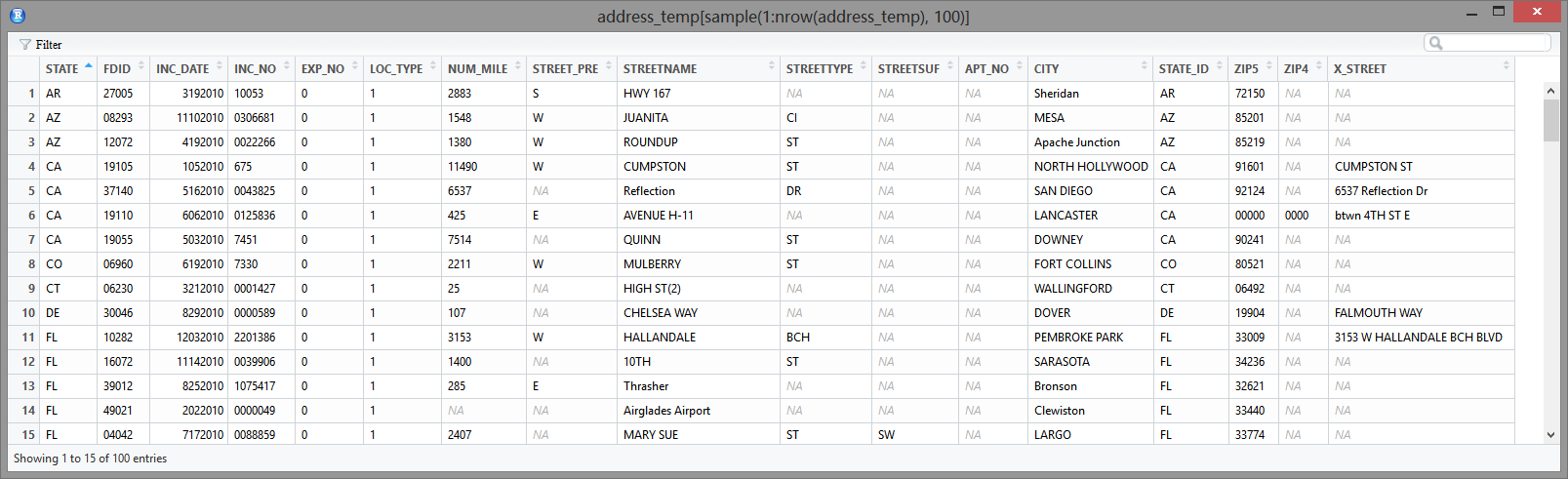
All the format errors
Here are the cleaning procedures I used. In the end I filtered and cleaned about 14% of data in many types.
# loading data and preparing address string
data_year = '2010'
# create year directory, load original address data, change year number here.
> head(str_subset(address$original_address, "N/A"))
[1] "55  Margaret ST  N/A, Monson, MA 01057"         "55  Margaret ST  N/A, Monson, MA 01057"
[3] "1657  WORCESTER RD   N/A, FRAMINGHAM, MA 01701" "132  UNION AV   N/A, FRAMINGHAM, MA 01702"
[5] "N/A  OAKLAND BEACH AV   , Warwick, RI 02889"    "00601  MERRITT 7 N/A  , NORWALK, CT 06850"

> head(str_subset(address$original_address, "null"))
[1] "96  Walworth ST  null, Saratoga Springs, NY 12866" "197 S Broadway   null, Saratoga Springs, NY 12866"
[3] "640  West Broadway   , Conconully, WA 98819"       "58  W Fork Rd   , Conconully, WA 98819"
[5] "  Mineral Hill Rd   , Conconully, WA 98819"        "225  Conconully ST  , OKANOGAN, WA 98840"
Because ‘NA’ or ‘na’ could be a valid part in address string, it’s better to clean them before concatenating fields into one address string.
> head(str_subset(address$original_address, "NA"))
[1] "7821 W CINNABAR AV  , PEORIA, AZ 00000"      "7818 W PINNACLE PEAK RD  , PEORIA, AZ 00000"
[3] "8828 W SANNA ST  , PEORIA, AZ 00000"         "8221 W DEANNA DR  , PEORIA, AZ 00000"
[5] "2026 W NANCY LN  , PHOENIX, AZ 00000"        "3548 E HELENA DR  , PHOENIX, AZ 00000"
Once I finished cleaning on fields, I will prepare a cleaner address string and do the further cleaning in that concatenated string. That’s why I concatenated all original fields into original_address, which is for reference in case some fields changed in later process.
Most other cleaning process are better done in the whole string, because some input may go to wrong fields, like street number in street name instead of street number column. With the whole string this kind of error doesn’t matter any more.
There are lots of usage of speical symobls like /, @, &, * in input which will interfere with the Geocoder.
> sample(address[LOC_TYPE == '1' & str_detect(address$input_address, "[/|@|&]"), input_address], 10)
 [1] "743 CHENANGO ST , BINGHAMTON/FENTON, NY 13901"             "123/127 tennyson , highland park, MI 48203"
 [3] "318 1/2 McMILLEN ST , Johnstown, PA 15902"                 "712 1/2 BURNSIDE DR , GARDEN CITY, KS 67846"
 [5] "m/m143 W Interstate 16 , Ellabell, GA 31308"               "12538 Greensbrook Forest DR , Houston / Sheldon, TX 77044"
 [7] "F/O 1179 CASTLEHILL AVE , New York City, NY 10462"         "509 1/2 N Court , Ottumwa, IA 52501"
 [9] "7945 Larson , Hereford/Palominas, AZ 85615"                "1022 1/2 N Langdon ST , MITCHELL, SD 57301"
First I remove all the 1/2 since the Geocoder cannot recognize them, and removing them will not affect the Geocoding result accuracy.
Many addresses used milepost numbers, which is a miles count along highway. They are not street addresses and cannot be processed by the Geocoder. There are all kinds of usage to record this type of address.
> head(str_subset(address$input_address, "(?i)milepost"))
[1] "452.2E NYS Thruway Milepost , Angola, NY 14006" "447.4W NYS Thruway Milepost , Angola, NY 14006"
[3] "446W NYS Thruway Milepost , Angola, NY 14006"   "447.4 NYS Thruway Milepost , Angola, NY 14006"
[5] "444.1W NYS Thruway Milepost , Angola, NY 14006" "I-94 MILEPOST 68 , Eau Claire, WI 54701"

> head(str_subset(address$input_address, "\\bmile\\b|\\bmiles\\b"))
[1] "2.5 mile Schillinger RD , T8R3 NBPP, ME 00000"        "cr 103(2 miles west of 717) , breckenridge, TX 00000"
[3] "Interstate 93 south mile mark , WINDHAM, NH 03087"    "183 lost mile rd. , parsonfield, ME 04047"
[5] "168 lost mile RD , w.newfield, ME 04095"              "20 mile stream rd , proctorsville, VT 05153"
Note it’s still possible to have some valid street address with mile as a word in address(my regular expression only check when mile is a whole word, not part of word), but it should be very rare and difficult to separate the valid addresses from the milepost usage. So I’ll just ignore all of them.
Another special format of address is grid style address. I decided to remove the grid number part and keep the rest of address. The Geocoder will get a rough location for that street or city, which is still helpful for my purpose. The Geocoding match score will separate this kind of rough match from the exact match of street addresses.
Grid-style Complete Address Numbers (Example: “N89W16758”). In certain communities in and around southern Wisconsin, Complete Address Numbers include a map grid cell reference preceding the Address Number. In the examples above, “N89W16758” should be read as “North 89, West 167, Address Number 58”. “W63N645” should be read as “West 63, North, Address Number 645.” The north and west values specify a locally-defined map grid cell with which the address is located. Local knowledge is needed to know when the grid reference stops and the Address Number begins. Page 37, United States Thoroughfare, Landmark, and Postal Address Data Standard
Most are WI and MN addresses. Except the E003 NY address, I’m not sure what does that means. Since the Geocoder cannot handle it either, they can be removed.
> sample(address[str_detect(address$input_address, "^[NSWEnswe]\\d"), input_address], 10)
 [1] "W26820 Shelly Lynn DR , Pewaukee, WI 53072"      "E14 GATE , St. Paul, MN 55111"
 [3] "W5336 Fairview ROAD , Monticello, WI 53570"      "W22870 Marjean LA , Pewaukee, WI 53072"
 [5] "E003 , New York City, NY 10011"                  "W15085 Appleton AVE , Menomonee Falls, WI 53051"
 [7] "N7324 Lake Knutson RD , Iola, WI 54945"          "N10729 Hwy 17 S. , Rhinelander, WI 54501"
 [9] "N2494 St. Hwy. 162 , La Crosse, WI 54601"        "N2639 Cty Hwy Z , Palmyra, WI 53156"
Some addresses have double quotes in it. Paired double quotes can be handled by the csv and Geocoder, but single double quote will cause problem for csv file.
> sample(address[str_detect(input_address, '"'), input_address], 10)
 [1] "317 IND \"C\" line at 14th ST , New York City, NY 10011" "750 W \"D\" AVE , Kingman, KS 67068"
 [3] "HWY \"32\" , SHEBOYGAN, WI 53083"                        "22796 \"H\" DR N , Marshall, MI 49068"
 [5] "5745 CR 631 \"C\" ST , Bushnell, FL 33513"               "CTY \"MM\" , HOWARDS GROVE, WI 53083"
 [7] "\"BB\" HWY , West Plains, MO 65775"                      "I-55 (MAIN TO HWY \"M\") , Imperial, MO 63052"
 [9] "3400 Wy\"East RD , Hood River, OR 97031"                 "6555 Hwy \"D\" , parma, MO 63870"
Some used ; to add additional information, which will only cause trouble for the Geocoder.
> sample(address[str_detect(input_address, ";"), input_address], 10)
 [1] "1816 MT WASHINGTON AV #1; WHIT , Colorado Springs, CO 80906"
 [2] "3201 E PLATTE AV; WAL-MART STO , Colorado Springs, CO 00000"
 [3] "1511 YUMA ST #2; CONOVER APART , Colorado Springs, CO 80909"
 [4] "3550 AFTERNOON CR; MSGT ROY P , Colorado Springs, CO 80910"
 [5] "805 S CIRCLE DR #B2; APOLLO PA , Colorado Springs, CO 00000"
 [6] "5590 POWERS CENTER PT; SEVEN E , Colorado Springs, CO 80920"
 [7] "715 CHEYENNE MEADOWS RD; DIAMO , Colorado Springs, CO 80906"
 [8] "3140 VAN TEYLINGEN DR #A; SIER , Colorado Springs, CO 00000"
 [9] "Meadow Rd; rifle clu , Hampden, OO 04444"
[10] "3301 E SKELLY DR;J , TULSA, OK 74105"
All these steps may look cumbersome. Actually I just check the Geocoding results on one year data raw input, find all the problems and errors, clean them by types. Then I apply same cleaning code to other years because they are very similar, and I got the Geocoding performance doubled! I think this cleaning is well worth the effort.
Version History
2016-02-03 : First version.
2016-05-11 : Added Summary.
]]>
<h2 id="Summary"><a href="#Summary" class="headerlink" title="Summary"></a>Summary</h2><ul>
<li>This is my second post on topic of Data Cleaning. </li>
<li>Cleaning addresses format turned out to have a substantial positive impact on Geocoding performance.</li>
<li>Deep understandings of address format standard is needed to deal with all kinds of special cases.</li>
</ul>
Data Cleaning Part 1 - NYC Taxi Trip Data, Looking For Stories Behind Errorshttps://dracodoc.github.io/2016/01/31/data-cleaning/2016-02-01T01:27:06.000Z2016-08-19T13:47:21.585ZSummary
Data cleaning is a cumbersome but important task for Data Science project in reality.
This is a discussion on my practice of data cleaning for NYC Taxi Trip data.
There are lots of domain knowledge, common sense and business thinking involved.
Data Cleaning, the unavoidable, time consuming, cumbersome nontrivial task
Data Science may sound fancy, but I saw many posts/blogs of data scientists complaining that much of their time were spending on data cleaning. From my own experience on several learning/volunteer projects, this step do require lots of time and much attention to details. However I often felt the abnormal or wrong data are actually more interesting. There must be some explanations behind the error, and that could be some interesting stories. Every time after I filtered some data with errors, I can have better understanding of the whole picture and estimate of the information content of the data set.
By the way, this analysis and exploration is pretty impressive. I think it’s partly because the author is NYC native and already have lots of possible pattern ideas in mind. For same reason I like to explore my local area of any national data to gain more understandings from the data. Besides, it turned out that you don’t even need a base map layer for the taxi pickup point map when you have enough data points. The pickup points themselves shaped all the streets and roads!
First I prepared and merged the two data file, trip data and trip fare.
library(data.table)
library(stringr)
library(lubridate)
library(geosphere)
library(ggplot2)
library(ggmap)
## ------------------ read and check data ---------------------------------
Some columns have obvious wrong values, like zero passenger count.
Though the other columns look perfectly normal. As long as you are not using passenger count information, I think these rows are still valid.
Another interesting phenomenon is the super short trip:
short = trip.all[trip_time_in_secs <10][order(total_amount)]
View(short)
One possible explanation I can imagine is that maybe some passengers get on taxi then get off immediately, so the time and distance is near zero and they paid the minimal fare of $2.5. Many rows do have zero for pickup or drop off location or almost same location for pick up and drop off.
Then how is the longer trip distance possible? Especially when most pick up and drop off coordinates are either zero or same location. Even if the taxi was stuck in traffic so there is no location change and trip distance recorded by the taximeter, the less than 10 seconds trip time still cannot be explained.
There are also quite some big value trip fares for very short trips. Most of them have pick up and drop off coordinates at zero or at same locations.
I don’t have good explanations for these phenomenon and I don’t want to make too many assumptions since I’m not really familiar with NYC taxi trips. I guess a NYC local probably can give some insights on them, and we can verify them with data.
Average driving speed
We can further verify the trip time/distance combination by checking the average driving speed. The near zero time or distance could cause too much variance in calculated driving speed. Considering the possible input error in time and distance, we can round up the time in seconds to minutes before calculating driving speed.
First check on the records that have very short time and nontrivial trip distance:
If the pick up and drop off coordinates are not empty, we can calculate the great-circle distance between the coordinates. The actual trip distance must be equal or bigger than this distance.
And there must be something wrong if the great-circle distance is much bigger than the trip distance. Note the data here is limited to the short trip time subset, but this type of error can happen in all records.
Either the taximeter had some errors in reporting trip distance, or the gps coordinates were wrong. Because all the trip time very short, I think it’s more likely to be the problem with gps coordinates. And the time and distance measurement should be much simpler and reliable than the gps coordinates measurement.
gps coordinates distribution
We can further check the accuracy of the gps coordinates by matching with NYC boundary. The code below is a simplified method which take center of NYC area then add 100 miles in four directions as the boundary. More sophisticated way is to use a shapefile, but it will be much slower in checking data points. Since the taxi trip actually can have at least one end outside of NYC area, I don’t think we need to be too strict on NYC area boundary.
I found another verification on gps coordinates when I was checking the trips started from the JFK airport. Note I used two reference points in JFK airport to better filter all the trips that originated from inside the airport and the immediate neighborhood of JFK exit.
# the official loc of JFK is too far on east, we choose 2 point to better represent possible pickup areas.
jfk.inside = data.frame(lon = -73.783074, lat = 40.64561)
jfk.exit = data.frame(lon = -73.798523, lat = 40.658439)
# rides from JFK could end at out of NYC, but there are too many obvious wrong gps information in that part of data, we will just use the data that have gps location in NYC area this time. This area is actually rather big, a square area with 200 miles edge.
# the actual distance threshold is adjusted by visual checking the map below, so that it includes most rides picked up from JFK, and excludes rides in neighborhood but not from JFK.
Interestingly, there are some pick up points in the airplane runway or the bay. These are obvious errors, actually I think gps coorindates report in big city could have all kinds of error.
Superman taxi driver
I also found some interesting records in checking taxi driver revenue.
So this driver were using different medallion with same hack license, picked up 1412 rides in March, some rides even started before last end(No.17, 18, 22 etc). The simplest explanation is that these records are not from one single driver.
rides = trip.march[, .N, by = hack_license]
summary(rides)
tail(rides[order(N)])
hack_license N
1: 74CC809D28AE726DDB32249C044DA4F8 1514
2: 51C1BE97280A80EBFA8DAD34E1956CF6 1530
3: 5C19018ED8557E5400F191D531411D89 1575
4: 847349F8845A667D9AC7CDEDD1C873CB 1602
5: F49FD0D84449AE7F72F3BC492CD6C754 1638
6: D85749E8852FCC66A990E40605607B2F 1649
These hack license owner picked up more than 1500 rides in March, that’s 50 per day.
We can further check if there is any time overlap between drop off and next pickup, or if the pick up location was too far from last drop off location, but I think there is no need to do that before I have better theory.
Summary
In this case I didn’t dig too much yet because I’m not really familiar with NYC taxi, but there are lots of interesting phenomenons already. We can know a lot about the quality of certain data fields from these errors.
In my other project, data cleaning is not just about digging interesting stories. It actually helped with the data process a lot. See more details in my next post.
Version History
2016-01-31 : First version.
2016-05-11 : Added Summary.
]]>
<h2 id="Summary"><a href="#Summary" class="headerlink" title="Summary"></a>Summary</h2><ul>
<li>Data cleaning is a cumbersome but important task for Data Science project in reality.</li>
<li>This is a discussion on my practice of data cleaning for NYC Taxi Trip data.</li>
<li>There are lots of domain knowledge, common sense and business thinking involved.</li>
</ul>
Script And Workflow For Batch Geocoding Millions Of Address With PostGIS Tiger Geocoderhttps://dracodoc.github.io/2015/11/19/Script-workflow/2015-11-19T20:05:00.000Z2016-08-19T19:39:10.803ZSummary
I discussed all the problem I met, approaches I tried, and improvement I achieved in the Geocoding task.
There are many subtle details, some open questions and areas can be improved.
The final working script and complete workflow are hosted in github.
Introduction
This is the detailed discussion of my script and workflow for geocoding NFIRS data. See background of project and the system setup in my previous posts.
So I have 18 million addresses like this, how can I geocode them into valid address, coordinates and map to census block?
Tiger Geocoder Geocode Function
Tiger Geocoder extension have this geocode function to take in address string then output a set of possible locations and coordinates. A perfect formated accurate address could have an exact match in 61ms, but if there are misspelling or other non-perfect input, it could take much longer time.
Since geocoding performance varies a lot depending on the case and I have 18 millions address to geocode, I need to take every possible measure to improve the performance and finish the task with less hours. I searched numerous discussions about improving performance and tried most of them.
Preparing Addresses
First I need to prepare my address input. Technically NFIRS data have a column of Location Type to separate street addresses, intersections and other type of input. I filtered the addresses with the street address type then further removed many rows that obviously are still intersections.
NFIRS designed many columns for different part of an address, like street prefix, suffix, apt number etc. I concatenate them into a string formated to meet the geocode function expectation. A good format with proper comma separation could make the geocode function’s work much easier. One bonus of concatenating the address segments is that some misplaced input columns will be corrected, for example some rows have the street number in street name column.
There are still numerous input errors, but I didn’t plan to clean up too much first. Because I don’t know what will cause problems before actually running the geocoding process . It will be probably easier to run one pass for one year’s data first, then collect all the formatting errors, clean them up and feed them for second pass. After this round I can use the clean up procedures to process other years’ data before geocoding.
Another tip I found about improving geocoding performance is to process one state at a time, maybe sort the address by zipcode. Because I want the postgresql server to cache everything needed for geocoding in RAM and avoid disk access as much as possible. With limited RAM it’s better to only process similar address at a time. Split huge data file into smaller tasks also make it easier to find problem or deal with exceptions, of course you will need a good batch processing workflow to process more input files.
Someone also mentioned that to standardize the address first, remove the invalid addresses since they take the most time to geocode. However I’m not sure how can I verify the valid address without actual geocoding. Some addresses are obviously missing street numbers and cannot have an exact location, but I may still need the ballpark location for my analysis. They may not be able to be mapped to census block, but a census tract mapping could still be helpful. After the first pass on one year’s data I will design a much more complete cleaning process, which could make the geocoding function’s job a little bit easier.
The PostGIS documentation did mention that the built-in address normalizer is not optimal and they have a better pagc address standardizer can be used. I tried to enable it in the linux setup but failed. It seemed that I need to reinstall postgresql since it is not included in the postgresql setup process of the ansible playbook. The newer version PostGIS 2.2.0 released in Oct, 2015 seemed to have “New high-speed native code address standardizer”, while the ansible playbook used PostgreSQL 9.3.10 and PostGIS 2.1.2 r12389. This is a direction I’ll explore later.
Test Geocoding Function
Based on the example given in geocode function documentation, I wrote my version of SQL command to geocode address like this:
SELECT g.rating,
pprint_addy(g.addy),
ST_X(g.geomout)::numeric(8,5) AS lon,
ST_Y(g.geomout)::numeric(8,5) AS lat,
g.geomout
FROM geocode('2198 Florida Ave NW, Washington, DC 20008', 1) AS g;
the 1 parameter in geocode function limit the output to single address with best rating, since we don’t have any other method to compare all the output.
rating is needed because I need to know the match score for result. 0 is for perfect match, and 100 is for very rough match which I probably will not use.
pprint_addy give a pretty print of address in format that people familiar.
geomout is the point geometry of the match. I want to save this because it is a more precise representation and I may need it for census block mapping.
lon and lat are the coordinates round up to 5 digits after dot. The 6th digit will be in range of 1 m. Since most street address locations are interpolated and can be off a lot, there is no point to keep more digits.
The next step is to make it work for many rows instead of just single input. I formated the addresses in R and wrote to csv file with this format:
row_seq
input_address
zip
42203
7365 RACE RD , HARMENS, MD 00000
00000
53948
37 Parking Ramp , Washington, DC 20001
20001
229
1315 5TH ST NW , WASHINGTON, DC 20001
20001
688
1014 11TH ST NE , WASHINGTON, DC 20001
20001
2599
100 RANDOLPH PL NW , WASHINGTON, DC 20001
20001
The row_seq is the unique id I assigned to every row so I can link the output back to the original table. zip is needed because I want to sort the addresses by zipcode. Another bonus is that addresses with obvious wrong zipcode will be shown together in beginning or ending of the file. I used the pipe symbol | as the separator of csv because there could be quotes and commas in columns.
Then I can read the csv into a table in postgresql database. The geocode function documentation provided an example to geocode addresses in batch mode, and most discussions in web seemed to be based on this example.
-- only update the first 3 addresses (323-704 ms
-- there are caching and shared memory effects so first geocode you do is always slower)
-- for large numbers of addresses you don't want to update all at once
LEFTJOIN (SELECT addid, (geocode(address,1)) AS geo
FROM addresses_to_geocode AS ag
WHERE ag.rating ISNULLORDERBY addid LIMIT3) AS g ON a.addid = g.addid
WHERE a.addid = addresses_to_geocode.addid;
Since the geocoding process can be slow, it’s suggested to process a small portion at a time. The address table was assigned an addid for each row as a index. The code always take the first 3 rows not yet processed (rating column is null) as the samplea to be geocoded.
SELECT addid
FROM addresses_to_geocode
WHERE rating ISNULLORDERBY addid LIMIT3) AS a
The result of geocodingg is joined with the addid of the samplea.
LEFT JOIN (SELECT addid, (geocode(address,1)) AS geo
FROM addresses_to_geocode AS ag
WHERE ag.rating ISNULLORDERBY addid LIMIT3
) AS g ON a.addid = g.addid
Then the address table was joined with that joined table a-g by addid and corresponding columns were updated.
The initial value of rating column is NULL. Valid geocoding match have a rating number range from 0 to around 100. Some input don’t have valid geocode function return value, which make the rating column to be NULL. Then it was replaced with -1 by the COALESCE function to be separated with the unprocessed rows, so that the next run can skip them.
The join of a and g may seem redundant at first since g already included the addid column. However when some rows has no match and no value is returned by geocode function, g will only have rows with return values. Joining g with address table will only update these rows by addid. COALESCE function will not take any effect since the empty row addid were not even included. Then the next run will select them again because they still satisfied the sample selection condition, which will mess up the control logic.
Instead joining a and g will have all addid in sample, and the no match rows have NULL in rating column. The next joining with address table will have the rating column updated correctly by COALESCE function.
This programming pattern is new for me. I think it’s because SQL don’t have the fine grade control of the regular procedure languages, but we still need more control some times so we have this.
Problem With Ill Formated Address
In my experiment with test data I found the example code above often had serious performance problems. It was very similar to another problem I observed: if I run this line with different table sizes, it should have similar performance since it is supposed to only process the first 3 rows.
SELECT geocode(address_string,1)
FROM address_sample LIMIT3;
Actually it took much, much longer on a larger table. It seemed that it was geocoding the whole table first, then only return the first 3 rows. If I subset the table more explicitly this problem disappeared:
SELECT geocode(sample.address_string, 1)
FROM (SELECT address_string
FROM address_sample LIMIT3
) assample;
I modified the example code similarly. Instead of using LIMIT directly in the WHERE clause,
SELECT addid, (geocode(address,1)) AS geo
FROM addresses_to_geocode AS ag
WHERE ag.rating ISNULLORDERBY addid LIMIT3
I explicitly select the sample rows then put it in the FROM clause, problem solved.
SELECT sample.addid, geocode(sample.input_address,1) AS geo
FROM (SELECT addid, input_address
FROM address_table WHERE rating ISNULL
ORDERBY addid LIMIT sample_size
) ASsample
Later I found this problem only occurs when the first row of table have invalid address for which the geocode function have no return value. These are the explain analysis results from pgAdmin SQL query tool:
The example code runs on 100 row table on first time, with first row address invalid. The first step of Seq Scan take 284 s (this was on my home pc server running on regular hard drive with all states data, so the performance was bad) to return 99 rows of geocoding result(one row has no match).
While my modified version only processed 3 rows in first step.
After the first row has been processed and marked with -1 in rating, the example code no longer have the problem
If I move the problematic row to the second row, there was no problem either. It seemed that the postgresql planner had some trouble only when the first row didn’t have valid return value. The geocode function authors didn’t find this bug probably because this is a special case, but it’s very common in my data. Because I sorted the addresses by zipcode, many ill formated addresses with invalid zipcode always appear in the beginning of the file.
Making A full Script
To have a better control of the whole process, I need some control structures from PL/pgSQL - sql procedural Language.
First I make the geocoding code as a geocode_sample function with the sample size for each run as parameter.
Create or replace make debugging and making changes easier because new version will replace existing version.
Then this main control function geocode_table will calculate the number of rows for whole table, decide how many sample runs it needed to update the whole table, then run the geocode_sample function in a loop with that number. I don’t want to use a conditional loop because if there is something wrong, the code could stuck at some point and have a endless loop. I’d rather just run the code with calculated times then check the table to make sure all rows are processed correctly.
DROPFUNCTIONIFEXISTS geocode_table();
CREATEORREPLACEFUNCTION geocode_table(
OUT table_size integer,
OUT remaining_rows integer) AS $func$
DECLARE sample_size integer;
BEGIN
SELECT reltuples::bigintINTO table_size
FROM pg_class
WHEREoid = 'public.address_table'::regclass;
sample_size := 1;
FOR i IN 1..(SELECT table_size / sample_size + 1) LOOP
PERFORM geocode_sample(sample_size);
ENDLOOP;
SELECTcount(*) INTO remaining_rows
FROM address_table WHERE rating ISNULL;
END
$func$ LANGUAGE plpgsql;
I used drop function if exists here because the Create or replace doesn’t work if the function return type was changed.
It’s widely acknowledged that calculating row count for a table by count(*) is not optimal. The method I used should be much quicker if the table statistics is up to date. I used to put a line of VACUUM ANALYZE after the table was constructed and csv data was imported, but in every run it reported that no update was needed. It probably because the default postgresql settings made sure the information is up to date right for my case.
In the end I counted the rows not processed yet. The total row number and the remaining row number will be the return value of this function.
The whole PL/pgSQL script is structured like this (actual details inside functions are omitted to have a clear view of whole picture. See complete scripts and everything else in my github repo):
DROPTABLEIFEXISTS address_table;
CREATETABLE address_table(
row_seq varchar(255),
input_address varchar(255),
zip varchar(255)
);
-- aws version.
COPY address_table FROM :input_file WITH DELIMITER '|' NULL 'NA' CSV HEADER;
-- pc version.
-- COPY address_table FROM 'e:\\Data\\1.csv' WITH DELIMITER ',' NULL 'NA' CSV HEADER;
ALTERTABLE address_table
ADD addid serialNOTNULL PRIMARY KEY,
ADD rating integer,
ADD lon numeric,
ADD lat numeric,
ADD output_address text,
ADD geomout geometry, -- a point geometry in NAD 83 long lat.
First I dropped the address table if previously exists, created the table with columns in characters type because I don’t want the leading zero in zipcode lost in converting to integer.
I have two version of importing csv into table, one for testing in windows pc, another one for AWS linux instance. The SQL copy command need the postgresql server user to have permission for the input file, so you need to make sure the folder permission is correct. The linux version used a parameter for input file path.
Then the necessary columns were added to table and the index was built.
The last line run the main control function and print the return value of it in the end, which is the total row number and remaining row number of input table.
Intersection address
Another type of input is intersections. Tiger Geocoder have a function Geocode_Intersection work like this:
FROM geocode_intersection( 'Haverford St','Germania St', 'MA', 'Boston', '02130',1);
It take two street names, state, city and zipcode then output multiple location candidates with ratings. The script of geocoding street addresses only need some minor changes on input table column format and function parameters to work on intersections. I’ll just post the finished whole script for reference after all discussions.
Map to Census Block
One important goal of my project is to map addresses to census block, then we can link the NFIRS data with other public data and produce much more powerful analysis, especially the American Housing Survey(AHS) and the American Community Survey(ACS).
There is a Get_Tract function in Tiger Geocoder which return the census tract id for a location. For census block mapping people seemed to be just using ST_Contains like this answer in stackexchange:
SELECT tabblock_id ASBlock,
substring(tabblock_id FROM1FOR11) AS Blockgroup,
substring(tabblock_id FROM1FOR9) AS Tract,
substring(tabblock_id FROM1FOR5) AS County,
substring(tabblock_id FROM1FOR2) AS STATE
FROM tabblock
WHERE ST_Contains(the_geom, ST_SetSRID(ST_Point(-71.101375, 42.31376), 4269))
The national data loaded by Tiger Geocoder have a table tabblock which have the information of census blocks. ST_Contains will test the spatial relationship between two geometries, in our case it will be whether polygon or multi polygon of census block contains the point of interest. The Where clause select the only record that satisfy this condition for the point.
The census block id is a 15 digits code constructed from state and county fips code, census tract id, blockgroup id and the census block number. The code example above actually are not ideal for me since it included all the prefix in each column. My code will work on the results from the geocoding script above:
UPDATE address_table
SET (tabblock_id, STATE, county, tractid)
= (COALESCE(ab.tabblock_id,'FFFF'),
substring(ab.tabblock_id FROM1FOR2),
substring(ab.tabblock_id FROM3FOR3),
substring(ab.tabblock_id FROM1FOR11)
)
FROM
(SELECT addid
FROM address_table
WHERE (geomout ISNOTNULL) AND (tabblock_id ISNULL)
ORDERBY addid LIMIT block_sample_size) AS a
LEFTJOIN (SELECT a.addid, b.tabblock_id
FROM address_table AS a, tabblock AS b
WHERE (geomout ISNOTNULL) AND (a.tabblock_id ISNULL)
AND ST_Contains(b.the_geom, ST_SetSRID(ST_Point(a.lon, a.lat), 4269))
ORDERBY addid LIMIT block_sample_size) AS ab ON a.addid = ab.addid
WHERE a.addid = address_table.addid;
I didn’t include the state fips as prefix in county fips since strictly speaking county fips is 3 digits, although you always need to use it with state fips together. I included the census tract because some location may have ambiguity but the census tract most likely will be same.
This code is based on same principle of the geocoding code with a little bit change:
It need to work on top of geocoding results, so the sample for each run are the rows that have been geocoded (thus geomout column is not NULL), but not yet mapped to census block (tabblock_id is NULL), and sorted by addid, limited by sample size.
Similar to geocode code, I need to join the sample addid with lookup result to make sure even the rows without return value are included in result. Then the NULL rating value of those rows will be replaced with an special value to mark the row as processed already but without match. This step is critical for the updating process to work properly.
In theory this mapping is much easier than geocoding since there is not much ambiguity. And every address should belong to some census block. Actually I found many street intersections don’t have matches. I tested the same address in the offcial Census website and it find the match!
Here is the example data I used, the geocode_intersection function returned a street address and coordinates from two streets:
row_seq        | 2716
street_1       |  FLORIDA AVE NW
street_2       | MASSACHUSETTS AVE NW
state          | DC
city           | WASHINGTON
zip            | 20008
addid          | 21
rating         | 3
lon            | -77.04879
lat            | 38.91150
output_address | 2198 Florida Ave NW, Washington, DC 20008
I used different test methods and found interesting results:
input
method
result
2 streets
geocode_intersection
(-77.04879, 38.91150)
geocode_intersection output address
geocode
(-77.04871, 38.91144)
geocode_intersection output address
Census website
(-77.048775,38.91151) GEOID: 110010055001010
geocode_intersection coordinates, 5 digits
Census website
census block GEOID: 110010041003022
geocode_intersection coordinates, 5 digits
Tiger Geocoder
census block GEOID: 110010041003022
geocode_intersection coordinates, 6 digits
Tiger Geocoder
census block: no match
If I feed the street address output from geocode_intersection back to geocode function, the coordinates output will have slight difference with the coordinates output from geocode_intersection. My theory is that geocode_intersection function first calculate the intersection point from the geometry information of two streets, then reverse geocode that coordinates into street address. The street number is usually interpolated so if you geocode that street address back to coordinates there could be difference. Update: Some interesting background information about the street address locations and ranges.
The slight difference may result in different census block output, probably because these locations are on street intersections which are more than likely to be boundary of census blocks.
Using the geometry or the coordinates output (6 digits after dot) from geocode_intersection for ST_Contains could have empty result, i.e. no census block have contain relationship of these points. I’m not sure the reason of this, only observed that using coordinates with 5 digits after dot will find a match in most time. This is an open question need to consulting with the experts on this.
Work In Batch
I was planning to geocode addresses by states to improve the performance, so I’ll need to process lots of files. After some experimentations, I developed a batch workflow:
The script discussed above can take a csv input, geocode addresses, map census block, update the table. I used this psql command line to execute the script. Note I have a .pgpass file in my user folder so I don’t need to write database password in the command line, and I saved a copy of the console messages to log file.
psql -d census -U postgres -h localhost -w -v input_file="'/home/ubuntu/geocode/address_input/address_sample.csv'" -f geocode_batch.sql 2>&1 | tee address.log
I need to save the result table to csv. The Copy in SQL require the postgresql user to have permission for output file, so I used the psql meta command \Copy instead. It can be written inside the PL/pgSQL script but I cannot make it to use parameter as output file name. So I have to write another psql command line:
psql -d census -U postgres -h localhost -w -c '\copy address_table to /home/ubuntu/geocode/address_output/1.csv csv header'
The above two lines will take care of one input file. If I put all input files into one folder, I can generate a shell script to process each input file with above command line. At first I tried to use shell script directly to read file names and loop with them, but it became very cumbersome and error prone because I want to generate output file name dynamically from input file names then transfer them as psql command line parameters. I ended up with a simple python script to generate the shell script I wanted.
Before running the shell script I need to change the permission:
chmod +x ./batch.sh
sh ./batch.sh
Exception Handling And Progress Report
The NFIRS data have many ill formated addresses that could cause problem for geocode function. I decided that it’s better to process one year’s data first, then collect all the problem cases and design a cleaning procedure before processing other years’ data.
This means the workflow should be able to skip on errors and mark the problems. The script above can handle the cases when there is no match returned from the geocode function, but any exception occurred in runtime will interrupt the script. Since the geocode_sample is called in a loop inside the main control function, the whole script is one single transaction. Once the transaction is interrupted, it will be rolled back and all the previous geocoding results are lost. See more about this.
However, adding an EXCEPTION clause effectively forms a subtransaction that can be rolled back without affecting the outer transaction.
Therefore I added this exception handling part in the geocode_sample function:
CREATE OR REPLACE FUNCTION geocode_sample(sample_size integer)
RETURNS void AS $$
DECLARE OUTPUT address_table%ROWTYPE;
BEGIN
...
EXCEPTION
WHEN OTHERS THEN
SELECT * INTO OUTPUT
FROM address_table
WHERE rating IS NULL ORDER BY addid LIMIT 1;
RAISE NOTICE '<address error> in samples started from: %', OUTPUT;
WHERE rating IS NULL ORDER BY addid LIMIT sample_size
) AS sample
WHERE sample.addid = address_table.addid;
END;
$$ LANGUAGE plpgsql;
This code will catch any exception, print the first row of current sample to notify the location of error, also print the original exception message.
psql:geocode_batch.sql:179: NOTICE:  <address error> in samples started from: (1501652," RIVER (AT BLOUNT CO) (140 , KNOXVILLE, TN 37922",37922,27556,,,,,,,,,)
CONTEXT:  SQL statement "SELECT geocode_sample(sample_size)"
PL/pgSQL function geocode_table() line 24 at PERFORM
psql:geocode_batch.sql:179: NOTICE:  -- !!! invalid regular expression: parentheses () not balanced 2201B !!!--
To make sure the script will continue work on the remaining rows, it also set the rating column of the current sample to be -2, thus they will be skipped in latter runs.
One catch of this method is the whole sample will be skipped even only one row in it caused problem, then I may need to check them again after one pass. However I didn’t find a better way to find the row caused the exception other than set up some marker for every row and keep updating it. Instead, I tested the performance with different sample size, i.e. how many rows will the geocode_sample function process in one run. It turned out sample size 1 didn’t have obvious performance penalty, maybe because the extra cost of small sample is negligible compared to the geocoding function cost. With a sample size 1 the exception handling code will always mark the problematic row only, and the code is much simpler.
Another important feature I want is progress report. If I split the NFIRS data by state, one state data often has tens of thousands of rows and take several hours to finish. I don’t want to find error or problem until it finishes. So I added some progress report like this:
psql:geocode_batch.sql:178: NOTICE:  > 2015-11-18 20:26:51+00 : Start on table of 10845
psql:geocode_batch.sql:178: NOTICE:  > time passed | address processed <<<< address left
psql:geocode_batch.sql:178: NOTICE:  > 00:00:54.3  |    100 <<<<    10745
psql:geocode_batch.sql:178: NOTICE:  > 00:00:21.7  |    200 <<<<    10645
First it report the size of whole table, then the time taken for every 100 rows processed, and how many rows are left. It’s pretty obvious in above example that the first 100 rows take more time. It’s because many address with ill formated zipcode were sorted on top.
Similarly, the mapping of census block have a progress report:
psql:geocode_batch.sql:178: NOTICE:  ==== start mapping census block ====
psql:geocode_batch.sql:178: NOTICE:  # time passed | address to block <<<< address left
psql:geocode_batch.sql:178: NOTICE:  # 00:00:02.6  |    1000    <<<<    9845
psql:geocode_batch.sql:178: NOTICE:  # 00:00:03.4  |    2000    <<<<    8845
My script has processed almost one year’s data, but I’m not really satisfied with the performance yet. When I tested the 44185 MD, DC addresses in the AWS free tier server with MD, DC database, the average time per row is about 60 ms, while the full server with all states have the average time of 342 ms. Some other states with more ill formated addresses have worse performance.
I have updated the Tiger database index and tuned the postgresql configurations. I can try parallel but the cpu should not be the bottle neck here, and the hack I found to enable postgresql run parallel is not easily manageable. Somebody also mentioned partitioning database, but I’m not sure if this will help.
And here are some open questions I will ask in PostGIS community, some of them may have the potential to further improve performance:
Why is a server with 2 states data much faster than the server with all states data? I assume it’s because the bad address that don’t have a exact hit at first will cost much more time when the geocoder checked all states. With only 2 states this search is limited and stopped much early. This can be further verified by comparing the performance of two test cases in each server, one with exact match perfect address, another one with lots of invalid addresses.
There is a restrict_region parameter in geocode function looks promising if it can limit the search range, since I have enough information or reason to believe the state information is correct. I wrote a query trying to use one state’s geometry as the limiting parameter:
SELECT geocode('501 Fairmount DR , Annapolis, MD 20137', 1, the_geom)
FROM tiger.state WHERE statefp = '24';
and compared the performance with the simple version
SELECT geocode('501 Fairmount DR , Annapolis, MD 20137',1);
I didn’t find performance gain with the parameter. Instead it lost the performance gain from caching, which usually came from running same query immediately again because all the needed data have been cached in RAM.
Maybe my usage is not proper, or this parameter is not intended to work as I expected. However if the search range can be limited, the performance gain could be substantial.
Will normalizing address first improve the performance? I don’t think it will help unless I can filter bad address and remove them from input totally, which may not be the case for my usage of NFIRS data. The new PostGIS 2.2.0 looks promising but the ansible playbook is not updated yet, and I haven’t have the chance to setup the server again by myself.
One possible improvement to my workflow is to try to separate bad formatted addresses with the good ones. I already separated some of them by sorting by zipcode, but there are some addresses with a valid zipcode are obviously incomplete. The most important reason of separate all input by state is to have the server cache all the data needed in RAM. If the server meet some bad formatted addresses in the middle of table and started to look up all states, the already loaded whole state cache could be messed up. Then the good addresses need the geocoder to read state data from hard drive again. If the cache update statistics could be summarized from the server log, this theory can be verified.
I’ve almost finished one year’s data. After it finished I’ll design more clean up procedures, and maybe move all suspicious addresses out to make sure the better shaped addresses geocoding are not interrupted.
Will replacing the default normalizing function with the Address Standardizer help? I didn’t find the normalizing step too time consuming in my experiments. However if it can produce better formated address from bad input, that could help the geocoding process.
Why 6 digits coordinates of street intersections output often don’t have matched census block, but coordinates round up to 5 digits have match in most of time?
Version History
2015-11-19 : First version.
2016-05-11 : Added Summary.
2016-08-19 : Syntax highlighting.
]]>
<h2 id="Summary"><a href="#Summary" class="headerlink" title="Summary"></a>Summary</h2><ul>
<li>I discussed all the problem I met, approaches I tried, and improvement I achieved in the Geocoding task.</li>
<li>There are many subtle details, some open questions and areas can be improved.</li>
<li>The final working script and complete workflow are hosted in <a href="https://github.com/dracodoc/Geocode" target="_blank" rel="external">github</a>.</li>
</ul>
Geocoding 18 million addresses with PostGIS Tiger Geocoderhttps://dracodoc.github.io/2015/11/17/Geocoding/2015-11-17T16:36:10.000Z2016-08-19T13:46:40.772ZSummary
This post discussed the background, approaches, windows and linux environment setup for my Geocoding task.
See more details about the script and workflow in next post.
Background
I found I want to geocode lots of addresses in my Red Cross Smoke Alarm Project. The NFIRS data have 18 million addresses in 9 years data, and I would like to
verify all the addresses because many inputs have quality problems.
map street address to coordinates, so we can map and do more geospatial analysis.
Online service. Most free online API have limit, and paid service would be too expensive for my task. Surprisingly FCC have an API to map coordinates to census block which didn’t mention limit, but it cannot geocode street address to coordinates.
Setup your own geocoder. Tiger geocoder is a PostGIS extension which use Census Tiger data to geocode addresses.
PostGIS can work in both windows and linux, and Enigma.io has shared their automated Tiger Geocoder setup tool for linux. However the Tiger database itself need 105G space and I don’t have a linux box for that(Amazon AWS free tier service only allow for 30G storage), so I decided to install PostGIS in windows and experiment with everything first.
Windows Setup
I need to install postgresql server, PostGIS extension and Tiger geocoder extension. This is a very detailed installation guide for PostGIS in windows. I’ll just add some notes from my experience:
It’s best if you could install the database in SSD drive. My first setup was in SSD and only have two states data, the geocoding performance was pretty good. Then I need to download all the states so I have to move the database to regular hard drive according to this guide (note the data folder path value cannot have the trialling escape, otherwise the PostgreSQL Service will just fail). After that the geocoding performance dropped considerably.
The pgAdmin is easy to use. I used SQL Query, View Data (or view top 100 rows if the table is huge) a lot. The explain analyze function in the SQL Query tool is also very intuitive.
With server and extension installed, I need to load Tiger data. The Tiger geocoder provided scripts generating functions for you to download Tiger data from Census ftp then set up the database. The official documentation didn’t provide enough information for me, so I have to search and tweak a lot. At first I tried the commands from SQL query tool but it didn’t show any result. Later I solved this problem with hints from this guide, although it was written for Ubuntu.
You need to install 7z.exe and wget windows version and record their path.
Create a directory for download. Postgresql need to have permission for that folder. I just created the folder in same level with the postgresql database folder, and both of them have user group Authenticated users in full control. If you write a sql copy command to read csv file in some other folder that don’t have this user permission, there could be a permission denied error.
Start pgAdmin, connect to the GIS database you created in installation, run psql tool from pgAdmin, input \a\t to set up format first, and set output file by
\o nation_generator.bat
then run
SELECT loader_generate_nation_script('windows');
to generate the script to load national tables. It will be a file with the name specified with \o nation_generator.bat before located in the same folder of psql.exe, which should be the postgresql bin folder.
Technically you can input the parameters specific to your system settings in the table loader_variables and loader_platform which are under tiger schema. However after I inputed the parameters, only the stage folder(i.e. where to download data to) was taken into generated script. My guess is the file path with spaces need be proper escaped and quoted. The script generating function is reading from database then write to file, hat means the file path will go through several different internal representations, which make the escaping and quoting more complicated. I just replaced the default parameters with mine in the generated script later. Update: I found this answer later. I probably should use SET command instead of directly editing the table columns. Anyway, replacing the settings afterwards still works, and you need to double check it.
All the parameters are listed in the first section of generated script, and cd your_stage_folder will be used several times through the script. You need to edit the parameters in first section and make sure the stage folder is correct in all places.
After the national data is loaded by running with the script, you can specify the states that you want to load. Actually the tiger database support 56 states/regions. You can find them by
select stusps, name from tiger.state order by stusps;
Start psql again, go through similar steps and run
Put the states abbreviations that you want in the array. Note if you copy the query results it will be quoted with double quote by default, but you need single quote in SQL. You can change the pgAdmin output setting in Options - Query tool - Results grid.
The generated script will have one section for each state, each section have parameters set in beginning. You need to replace the parameters and the cd your_stage_folder to correct values. Using an editor that support multi line search replace will make this much easier.
I don’t want to load 56 states in one script. If anything went wrong it will be bothersome to start again from last point. I wanted to split the big script into 56 ones, one state each. I searched for a while and didn’t find a software to do this, then I just wrote a python script.
First add a marker in the script to separate states. I replaced all occurrences of
set TMPDIR=e:\data\gisdata\temp\\
to
:: ---- end state ----
set TMPDIR=e:\data\gisdata\temp\\
then deleted the :: ---- end state ---- marker in the first line. This make the marker appear in the end of each state section. Note the :: is commenting symbol in dos bat so it will not interfere with the script.
Then I run this python script to split it by states.
After I moved the postgresql database to regular hard drive because of storage limit, the geocoding performance was very low. Fortunately I got the generous support of DataKind on their AWS resources, so I can run the geocoding task in Amazon EC2 server. I want to test everything as comprehensive as possible before deploying an expensive EC2 instance, thus I decided to do everything with the Amazon EC2 free tier service first. The free tier only allow 30G storage, 1G RAM but I can test with 2 states first.
I used the ansible playbook from Enigma to setup the AWS EC2 instance. Here are some notes:
Be careful when using AWS free tier service, anything not explicitly marked as free tier could cost money.
For a test server with national tables and 2 states data, the free tier t2.micro instance actually is enough. You can normalizing addresses, mapping census block for all states and geocoding for those 2 states addresses. Actually my 2 states free server with 1G RAM is much faster than the t2.large 8G server with all states data loaded. I’ll discuss this in more details in another post about the geocoding script.
I used bitvise as my ssh and sftp tool since it seemed to be an enhanced putty.
I either use nano as the editor in AWS instance (for error with nano history), or just download the file to be edited with sftp, edit then upload (sometimes I may need to convert the script with dos2unix). It’s much easier to edit multiple places with sublime.
After lots of experimentation I have my batch geocoding workflow ready, then I started to setup the full scale server with DataKind resources.
Interestingly, sudo doesn’t work in the t2.large instance. I searched and found it’s because the private ip is not in hosts. The problem can be solved by adding the machine name into hosts file, however how can you edit hots file without sudo? Finally I used this to solve this problem.
sudo passwd root
su root
nano /etc/hosts
su ubuntu
The command of running ansible playbook from the Enigma repo have \ to extend one line into multiple lines. My first try didn’t copy the new line after each \ correctly (because I was using a firefox extension to automatically copy on select) and the command cannot run, but the error message was very misleading so I didn’t realize it’s because of this.
Although the Tiger database will take 105G at last, the downloading and provisioning need more spaces for temporary files. My first attempt with 120G storage was filled up in the provisioning, so I have to start again with 180G.
Gnu Screen let you use same terminal window to switch between tasks or even split windows, so that you can leave the process running but detached from the screen. It’s essential to run and control the time consuming tasks. Here is a cheat sheet and quick list.
I enabled the color prompt of bash by removing comment of #force_color_prompt=yes in ~/.bashrc. When you need to scroll through long history of command line or reading many lines of output, a colored prompt could separate the command and the output well.
You may need to use psql a lot, so I placed a .pgpass file in my user folder (change its permission with chmod 0600 ~/.pgpass). I also set several other options in .psqlrc file in user folder, including color prompt, timing on, vertical output etc.
\timing
\x auto
\set COMP_KEYWORD_CASE upper
\set PROMPT1 '%[%033[1;33;40m%]%n@%/%R%[%033[0m%]%# '
I was not satisfied with the geocoding performance so I experimented with tuning postgresql configurations. This post and this guide helped me most. The average time needed for geocoding one address in a 200 records sample dropped from 320 ms to 100 ms.
Geocoding Script And Work Flow Setup
I’ll discuss the geocoding script and my work flow for batch geocoding in next post.
Version History
2015-11-17 : First version.
2016-05-11 : Added Summary.
]]>
<h2 id="Summary"><a href="#Summary" class="headerlink" title="Summary"></a>Summary</h2><ul>
<li>This post discussed the background, approaches, windows and linux environment setup for my Geocoding task.</li>
<li>See more details about the script and workflow in next post.</li>
</ul>
Red Cross Smoke Alarm Projecthttps://dracodoc.github.io/2015/11/11/Red-Cross-Smoke-Alarm-Project/2015-11-11T14:02:10.000Z2016-08-19T13:48:32.625ZSummary
This is a write-up for my volunteer Data Science project for the American Red Cross.
The project used public data to help Red Cross directing limited resources to homes that more vulnerable to fire risk and loss.
My work in the project:
Discovered the hidden information in NFIRS dataset, obtained and analyzed 10G NFIRS data.
Major contribution on model design, implemented NFIRS related predictors, and built interactive visualizations.
Geocoded 18 millions address in NFIRS data with AWS server, Postgresql, PostGIS.
The choropleth map of Red Cross Smoke Alarm Home Visits per county in 10 months
Project Goal
Given limited resources and the ambitious project goal, the American Red Cross want to have a priority list for regions backed with data and analysis. The ranking could came from multiple factors, like the possibility of don’t have smoke alarm installed, the risk of catching fire, the possible casualty and losses, maybe even taking the constraints of each Red Cross chapter into consideration.
They first targeted the areas of least likely to have smoke alarm installed. The American Housing Survey(AHS) provided some data on this in county level, and the American Community Survey(ACS) have more detailed results about many other questions in census block group level. Using the shared questions in these two survey, they were able to build a model to predict smoke alarm presence in block group level, thus same number of home visits could cover more homes without smoke alarms.
Then they studied the areas of most likely to suffer structure fire fatalities. According to NFPA research, very young and very old are most susceptible to fire fatalities. Thus they calculated the fire risk per housing unit according to New Orleans historical data, then added age adjustment based on census population data. With these two factors combined, they ranked the high priority regions for smoke alarm outreach program.
After this New Orleans program, Enigma.io further expanded the acs/ahs method to national level, and produced a visualization website showing risk of lacking smoke alarms on map. They don’t have fire risk data in national level, but provided an API to upload local fire risk data into the model.
More Data Sources
The American Red Cross project is a national level campaign in much larger scale compared to New Orleans project. Red Cross provided the data of their smoke alarm home visits in 10 months and the data of Red Cross disaster response to us for our analysis.
The American Red Cross Diaster response for fire per county
They also got several years National Fire Incident Reporting System (NFIRS) data, listed every fire incident’s time and address. These were the starting point for us to work on.
I found the NFIRS data promising since it is the most complete public data set of fire incidents on national level. After lots of time spending on documents and search, I found this data set is very rich in information, although the problems and challenges are huge too.
The Fire Incidents reported by NFIRS per county in 2010
The Fire Incidents reported by NFIRS per ZCTA of Maryland in 2010
First, the original NFIRS data included many aspects of fire incident, including time, location, fire type, cause of fire, whether there was fire detectors, whether the detectors alerted occupants, the casualty and property losses etc, the list could go on and on. The dataset we got from Red Cross is a compiled version with every address geocoded and verified, which are very useful. However I want to dig more information from the source.
The U.S. Fire Administration website said you can order cd-rom from them for NFIRS data. However I searched and found some direct download links from FEMA. I downloaded all the data I found, from 1999 to 2011. Unfortunately, later I found the data of 2002 ~ 2009 only have about half the states. I guess it’s because the data are excel files and each worksheet in excel can only hold 1 million rows, so the other half states were missing. Fortunately I contacted USFA and they sent the cd-roms of 2005 ~ 2013 to me, now we have 9 years complete and more recent data!
Problems and Challenges
Using NFIRS data is not easy. Their website stressed again and again that you should not just count the incidents, because NFIRS participation is not mandatory at the national level. With about 2/3 of all fire departments participating, it only included about 75% of all reported fires. To make things worse, there is no definitive list of all fire departments and the participating departments. There are some very limited fire department census data, and some fire department data for each year which are not up to date for all the changes in fire departments. How to adjust for this coverage bias is a big challenge.
Another widespread problem is the data quality. There are many columns not filled, data recorded in wrong column and obvious input errors (some years’ data even excluded Puerto Rico entirely because of data quality problems).
Besides, the fire detectors defined by NFIRS including other type of alarms beside smoke alarm. Although there are further break down of detector types, but the valid entries only take 10 ~ 20 % in all home fires records.
In the research on all these problems, I found many analysis methods will need to have the fire incident address geocoded, i.e. verify the address, get the coordinates and map to census block. This is the basis of linking NFIRS data with other data, or doing any geospatial analysis.
Geocoding 18 million addresses
The NFIRS data have 20 million incidents each year. The public data only includes fire incidents, that’s still 2 million each year and I have 9 years of data. Actually we should be only interested in home fires which is a part of all fire incidents, but I think the complete incidents location distribution can help to estimate the NFIRS data coverage, so I still want to geocode all incidents addresses. This geocoding task is impossible for any free online service and too expensive for any paid service. I have to setup a geocoding server by my own.
The data and the software needed are all public and free, though it is definitely not a trivial task. Enigma.io open sourced their geocoding server setup as an ansible playbook, but that’s for Amazon EC2, local linux machine or linux virtual machine. I’m using windows and afraid of the performance limit of virtual machine, so I still need to install everything and setup everything in windows.
After some efforts I got the server running with just 2 states data to test. Then it’s SQL time. With lots of learning, experiments I finally got a working script. The experiments were promising, however I have to move the database out of the SSD drive when I started to download full national data which amount to 100G. With all the data downloaded in regular hard drive, I found the geocoding performance deteriorated seriously, which make the geocoding task very time consuming.
Fortunately I got the generous support of DataKind on their AWS resources, now I can run the geocoding task in Amazon EC2 server. I want to test everything as comprehensive as possible before deploying an expensive EC2 instance, so I decided to do everything with the Amazon EC2 free tier service first. The free tier only allow 30G storage, 1G RAM but I can test with 2 states first.
Now I can use the ansible playbook from Engima. With some tweak I got it running with 2 states data. Surprisly the performance is much better than home pc, even with just 1G RAM. Though I’m not sure if the geocoding peformance will drop again with full national data downloaded.
I further improved my script to make it work with big input file and can work in batch mode. I found I have to use a mix of SQL, plpgsql, shell, python to get a fully batch mode work flow. I’ll write about the geocoding server setup and share my script later. I probably searched hundreds of questions, read hundreds of documentation, and made stackoverflow my most frequent visit site. So it will be a very long post.
My next step is to setup a full scale Amazon EC2 server to geocode all NFIRS data and other possible candidates. With all the address geocoded, we can do lots of things and link to many other data sources, it will be very promising.
Update: Interactively visualizing fire incident by population for each census tract
Update: I have finished the Geocoding and built indicators based on the accurate location of NFIRS events. Here are some sample interactive visualization of the results. You can zoom in and click any census tract for more details.
Reported structured fire incidents per 1000 people for each census tract in Maryland
2009
2010
2011
2012
2013
Version History
2015-11-11 : First version.
2016-05-10 : Added Summary.
2016-05-11 : Added visualization of fire incident per census tract.
]]>
<h2 id="Summary"><a href="#Summary" class="headerlink" title="Summary"></a>Summary</h2><ul>
<li>This is a write-up for my volunteer Data Science project for the American Red Cross.</li>
<li>The project used public data to help Red Cross directing limited resources to homes that more vulnerable to fire risk and loss.</li>
<li>My work in the project:<ul>
<li>Discovered the hidden information in NFIRS dataset, obtained and analyzed 10G NFIRS data.</li>
<li>Major contribution on model design, implemented NFIRS related predictors, and built interactive visualizations.</li>
<li>Geocoded 18 millions address in NFIRS data with AWS server, Postgresql, PostGIS.</li>
</ul>
</li>
</ul>
Exploring House Price Estimation And Imagining A Better Real Estate Websitehttps://dracodoc.github.io/2015/10/23/house-price/2015-10-23T18:23:53.000Z2016-08-19T13:53:27.004ZSummary
This personal project was inspired by my own experience in housing market. I was wondering what I can achieve with public data and Data Science methods.
Built upon extensive research of domain knowledge, my model is very simple yet powerful. It used the data with most information, followed the trends in space and time.
The prediction accuracy is comparable to Zillow Zestimate, although I don’t really think this accuracy number matters too much. The variation is still too large which is in part due to the nature of house sale/bid process.
Instead of trying to improve prediction accuracy numbers, I think it is more practical to list more reasonable comparable sales to user.
Introduction
I was looking at local housing market some time ago and found it was difficult to judge how much a house worth or how much it will be sold at. Real State agents could have a very good estimate based on their experience, but it is really an overwhelming problem for first time home buyer or seller.
There are many aspects about a house that could affect how much it worth to buyer. And every buyer has different preference and priorities about these aspects.
Only a subset of all possible buyers will see the house listing and consider it seriously. The actual candidate buyer pool is small and very susceptible to random factors like timing and other details.
The negotiations involve more random events and human decisions.
Naturally I searched for house price estimation tool on line. The best and most complete one is Zillow.com’s Zestimate®. Using huge amount of data for more than 100 million homes and sophisticated algorithms to estimate house sale price. Their performance? Estimation within 20% of sale price in 81.4% of times. Take a $500,000 house as example, that means $100,000 error.
The formal house price assessment procedures
Not satisfied with this kind of accuracy, I did some research on house price evaluation principles. I found two formal house price assessment procedures provided some insight:
Home owner insurance companies have a complex model to estimate cost of rebuilding the same house. The model require customer to report lots of detailed information about the house features and conditions. Sometimes insurance company will also send a professional inspector. The home owner insurance estimate doesn’t include the cost of land.
To establish base for property tax, county government assess the value of house from time to time. Maryland utilized a combination of two methods to assess the fair market value of a house. Cost approach is similar to insurance company that calculated the rebuild cost but added the land cost. Sales approach use the sale price of comparable properties. It was said that they use Cost approach for house cost and Sales approach for land cost, maybe because the county have the information of land cost for real estate developers. Though I have seen lots of houses in same area have same land cost even their area vary a lot.
I can’t really use Cost approach since I don’t have the insurance company model, and the public available information for individual house are very limited and often have many errors, far less and worse than the data that insurance company can get.
Sales approach looks more promising since fair market price actually included all the information of house build cost and market trends. It may sound good, but where are comparable sales? There are no identical properties, all the reference sales must have some difference in features, time, location etc. To calculate these differences into price, we are back facing the original assessment problem again.
My analysis of house price
After some research, exploring data with programs, and my own experience in negotiations, my understandings and assumptions of house price are as follows:
House sale price is the result of negotiations between seller and buyer. They make the decision based on their estimates on several things:
His/her own perspective. How much does it worth in his/her view? This include both objective features and subjective preferences.
His/her estimate of the opponent in negotiation. People will only make offer/counter offer at a level that they believe it’s possible to be accepted, at least in final round of negotiation. Knowing more about the house condition and the opponent’s situation can help a lot.
There are many other factors contribute to the above two, including national and local market trends, other opinion sources like agent, the timing of everything etc.
This may seem very subjective and impossible to predict. I don’t expect public data or any model can predict each individual’s personal preference, emotional factors, all the other random events. Even if a perfect prediction on sale price exists, once it was known it will immediately push the negotiations away from the prediction.
The individual buyer/seller perspective may keep unknown, however the overall result of sales in general are more predictable because the comparable sales in market are very strong references that both side will use to establish their perspective. If there are some very comparable recent sales and they expect to have similar sales in near future(the time and location distribution are both important, sales happened long time ago are not really comparable anymore), they knew they must align their expectations with these reference points.
If the reference price is higher, seller can always expect similar high price and continue to wait for other buyer.
If the reference price is lower, buyer can always move on and believe there will be a similar sale at lower price.
The other side of negotiations also knew this and have to accept the market situations.
Thus I can try to establish an estimate on fair market value based on comparable sales, which can be very helpful to home buyer and seller as a good base point, not exactly prediction of final sale price.
How to measure prediction accuracy
Now it’s easier to understand why Zestimate accuracy is not that impressive, because there are too many random events of each sale cannot be predicted with publicly available data. Actually I think it will be better to just predict a fair market value and give a estimate of variation range. A specific value may look like more accurate, but the buyer/seller will not really trust it because of the big margin of error. A core value plus a range will provide more information and give buyer/seller better understanding about the house price.
Zestimate did give a value range, and the range could be narrower when there are more information available for the house, for example house in metro area could have a 10% value range instead of national average of 20%. This is understandable since more comparable sales provided more “anchors” and the variation will be small according to our analysis above.
The Zestimate accuracy for different regions also showed this effect, where Delaware is much easier to predict than Alaska. Although their houses in market are in same level, but Delaware houses must be much more dense so there will be more comparable sales for each house.
I also observed that there are very big accuracy differences among metro areas, even they all suppose to have sufficient information.
My guess is that areas that are in fast changing phase or with more diversity will be more difficult to predict than areas in stable phase. Because of the diversity and fast changes, the actual comparable sales amount is not really big. If you divide that area into smaller sections to reduce diversity and variation, the scale of data points also dropped. Thus the 4.9 millions homes in NY may not provide more comparable sales information than the 681,000 homes in Las Vegas.
Based on above findings, I adjusted my project goal from estimate house sale price to estimate fair market value and variation range. Note the fair market value in my definition is not really an objective intrinsic value. It reflected the information we can decode from the market, and the variation range cover all the factors we cannot account for. With more information — mainly comparable sales — we can have less unknown and reduce the variation range. Ideally if there are many comparable sales happened nearby and recently, these sales and the next house sale are more likely to fall in a pretty narrow range.
Comparable sales in details
Comparison implies distance. If we look at the comparable sales in depth, there are at least 3 dimensions to define distance and similarity:
House feature. This is obvious but not easy. Everybody have his/her own preference, and the importance of house feature needed to considered under context. If there are many acceptable options, buyer could be more picky about house. However if there is not much option available, even non-perfect house features may have to be ignored.
Location. This is another obvious dimension but it also mean different for different people:
School district for family with needs.
Commute and public transportation options and cost.
Regional development which impact the house resale value in future.
Some people also will consider the more detailed level of location like the specific location and environment in community.
Time. More recent sales are more relevant. Depend on seller/buyer’s acceptable time span for house transaction, the length of relevant period could vary from days to months.
All the sales should be measured in these 3 dimensions to compare their similarity. These dimensions are based on objective data but have different meanings to different people. We cannot calculate each individual’s preference but we can segment people into some major groups in each dimension. For example
School district may be top priority for some families, while young family without kids may consider transportation first.
Investment property buyer will look at regional development and market condition.
Imagine a better real estate website: recommend houses for home buyer, list comparable sales for home buyer/seller
In the analysis of comparable sales I found there are lots of information can be useful to home buyer/seller and cannot be consolidated into a single number. My project goal of fair market value and variation range also need more context to be really meaningful.
I’m no longer focusing on trying to produce a house price number with high accuracy any more. I think it’s a impossible and meaningless mission. The data analysis and modeling in my imagination could provide great help to home buyer/seller by giving a full list and match scores instead of a single number:
Collect data from home seller/buyer for their preference and groups.
Based on available public data, filter houses for home buyer. I didn’t say “ideal house” because it either non-exist or too expensive and out of budget, which equal to non-exist. I also don’t think a single match score will represent all the dimensions of house. This could be a better visual tool to show the buyer’s expectation and the house’s actual score in each dimension:
The reason to make it more complicate than a single number is that people’s preference can change in different context. They may adjust the weights of dimensions according to the limit of available options or any new information. Thus a multi dimensional comparison will be more adaptive and useful.
I used some real estate websites a lot in my own experience as a customer and in my research. They sure can recommend “similar houses” for the property you have interest, but the recommendation quality often cannot meet my expectation. These websites also provide lots of filter conditions in house search, however the specific sqft value range or bedroom numbers are just the easiest data point to measure, not the best guides of how people compare houses.
List comparable sales for home buyer/seller. They will work as reference points for them to build a more accurate perspective and understanding of market. Because house sale involve multiple parties, they need to know not only the comparable sales in their own view, but also the comparable sales in the other party’s view. Of course if the preference is not public, they can only either guess the group the other party belong to or use the most general big group to estimate. These expectations are the corner stones of negotiation, thus very important in shaping the final sale price.
I believe the negotiations and the house sale could be more efficient with more information and shared reference points, and this could lead to a better market.
Back to data and analysis
I haven’t talk about much data yet in this post about Data Science. Actually I started to collect data in the very beginning in my research, but I want to have a better understanding about the problem, so I did more research, explored the data with R program, with just checking individual records by hand, try to understand the logic behind the results, built models and tested the prediction performance, then back to do more research about the problem. The theory above is the final product of a long series of research, exploring, thinking and experiments.
I have much more ideas than my time for implementation, actually my current model is just one of the simplest form:
For any house, based on its tax assessment value, apply the moving average sales/tax assessment ratio of recent, nearby house sales.
The performance of this simple model is not bad at all:
Zillow Zestimate
My Model
National, within 20%
78.3 %
NA
Maryland, within 20%
76.8 %
NA
My 3k dataset since 2014, within 20%
91.87 %
92.58%
My 3k dataset since 2014, within 10%
76.47 %
65.82%
The performance of my simple model and Zillow Zestimate on same dataset of 3000 homes. The estimation errors are divided by the sale price, this is the metric used by Zillow to measure Zestimate accuracy.
The National and Maryland Zestimate accuracy number was taken on July, 2015. The specific Zestimate values on the dataset were downloaded from April to July. The most current Zestimate values and performance statistics may have been updated.
Version History
2015-10-23 : First version.
2016-05-10 : Added Summary.
]]>
<h2 id="Summary"><a href="#Summary" class="headerlink" title="Summary"></a>Summary</h2><ul>
<li>This personal project was inspired by my own experience in housing market. I was wondering what I can achieve with public data and Data Science methods.</li>
<li>Built upon extensive research of domain knowledge, my model is very simple yet powerful. It used the data with most information, followed the trends in space and time.</li>
<li>The prediction accuracy is comparable to Zillow Zestimate, although I don’t really think this accuracy number matters too much. The variation is still too large which is in part due to the nature of house sale/bid process.</li>
<li>Instead of trying to improve prediction accuracy numbers, I think it is more practical to list more reasonable comparable sales to user.</li>
</ul>
Simple Python performance timing by checkpointshttps://dracodoc.github.io/2015/10/20/simple-python-performance-timing-by-checkpoints/2015-10-21T00:16:43.000Z2016-08-19T19:09:47.192ZSummary
This is a simple python script that can measure python program running time in fine levels.
It’s simpler than a full profiler, easier to use than other currently available similar scripts.
The need of a simple timing script
I have been revisiting Python recently and walked through Google’s tutorial. Interestingly my first solution to one of the exercise word count took a lot of time to analysis a 600K text.
I wanted some profile tool to locate the bottle neck. There are lots of profiler tools but they seemed to be too “heavy weighted” for my simple purpose. This great Python profiler guide introduced a simple timing context manager script to measure script execution. You will need to
wrap blocks of code that you want to time with Python’s with keyword and this Timer context manager. It will take care of starting the timer when your code block begins execution and stopping the timer when your code block ends.
Like this
from timer import Timer
from redis import Redis
rdb = Redis()
with Timer() as t:
rdb.lpush("foo", "bar")
print"=> elasped lpush: %s s" % t.secs
with Timer() as t:
rdb.lpop("foo")
print"=> elasped lpop: %s s" % t.secs
I used this method and found out the problem in my script is that I used
if key in dict.keys()
which seems natural since I saw this before:
for key in sorted(dict.keys()):
However, this is a linear look up in a list which didn’t utilize the constant time access of HashMap. The right way is to use dict directly without keys().
if key in dict
So the problem was solved but I still found the timing context manager not simple and intuitive enough. Adding timer means lots of edits and indents of original code, and moving checkpoints involves more editing and indenting.
My version of an even simpler timing script
Therefore, I wrote a simple script that have similar function of timing code blocks by checkpoints, also kept the usage effort minimal.
import the script
Place times.start(digit) in the place that you want the timer start. digit control the digits after the decimal point, default at 7.
Use times.seg_start("msg") and times.seg_stop("msg") enclose a code block and print the time of start and stop. msg can be used to identify the code block in the output.
You can also add single checkpoint times.last_seg anywhere, it will print the time elapsed since last checkpoint which could be of any type.
Here is an example of using timing script in Wordcount. You can search and highlight times to see all the edits needed in script.
print"==>| %.*f s" % (Digit[0], total), 'Total time elapsed'
Of course sometimes you want more features like execution frequency and memory analysis, then you can always use more powerful profiler like line_profiler and memory profiler. The profiler guide I mentioned earlier have detailed introductions on them.
That being said, I still found my simple timing script is often useful enough and easy to use with minimal overhead.
2015-10-20 : Some edits when I moved my blog to github pages.
2016-05-10 : Added Summary.
2016-08-19 : Syntax highlighting for all code chunks
]]>
<h2 id="Summary"><a href="#Summary" class="headerlink" title="Summary"></a>Summary</h2><ul>
<li>This is a simple python script that can measure python program running time in fine levels. </li>
<li>It’s simpler than a full profiler, easier to use than other currently available similar scripts.</li>
</ul>